Section 1.1 Types of Variables and their Relationships (B1)
When one does statistics, what is it exactly that we are observing and measuring? What are we computing?
In this section, we recognize different types of variables and classify them, and describe potential relationships between variables in a data set.
Exploration 1.1.1. Hours of sleep.
In this introductory activity, we ask ourselves some natural questions that one would ask when collecting and analyzing data.
(a)
As a class write down the average time (in hours, to the nearest half-hour) they sleep per night.
(b)
Then create a simple graph (called a dot plot) of the data. For example, consider the following data:
The dot plot for this data would be as follows: 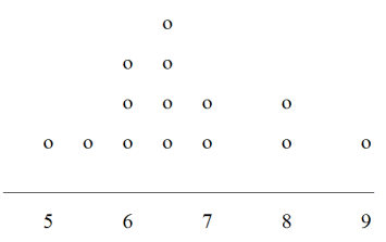
(c)
Does your dot plot look the same as or different from the example? Why?
(d)
If you did the same exercise in an English class with the same number of students, do you think the results would be the same? Why or why not?
(e)
Where do your data appear to cluster? How could you interpret the clustering?
(f)
What could we say about the Average Sleeping time of other students at your school? Would it matter if they were taking Statistics? Why or why not?
(g)
What are some reasons one may doubt the conclusions you've reached?
Congratulations! You're on your way to becoming a Statistician.
Definition 1.1.2.
Descriptive Statsitics is the organization and summary of data.
Inferential Statistics is using data to infer conclusions, and assesing the relative confidence we can state those conclusions
Subsection 1.1.1 Types of Variables
When we do either descriptive or inferential statistics, we are describing or infering properties of variables. Variables come in two types, each with two subcategories.
Definition 1.1.3.
-
Numerical variables are variables who's values are representable as numbers which can meaningfully be summed, subtracted or averaged.
Discrete variables have values spaced out by regular units, typically whole number value.
Continuous variables have values where number between values are also potential values.
-
Categorical variables have values that are categories rather than numerical.
Ordinal variables have values which have a natural ranking.
Nominal variables do not exhibit a natural ranking.
Activity 1.1.2. Classifying Variables.
(a)
For each of the following, classify the variable type and subcategory.
The colors of crayons in a 24-crayon box.
Student ID Numbers.
Grade Point Averages.
Pounds of fish caught on a fishing trip.
Number of fish caught on a fishing trip.
Year of Birth.
Annual income in dollars.
A satisfaction survey of a social website by number: 1 = very satisfied, 2 = somewhat satisfied, 3 = not satisfied.
(b)
Then, for each of the four subcategories, come up with two additional examples.
Activity 1.1.3. Classifying Variables from a Data Set.
In this activity, we look at an actual sample of data.
Run the following code to download the heart_transplant.csv data and to display it.
(a)
Run names(heart_transplant) to see just the variable names.
id - ID number of the patient.
acceptyear - Year of acceptance as a heart transplant candidate.
age - Age of the patient at the beginning of the study.
survived - Survival status with levels alive and dead.
survtime - Number of days patients were alive after the date they were determined to be a candidate for a heart transplant until the termination date of the study
prior - Whether or not the patient had prior surgery with levels yes and no.
transplant - Transplant status with levels control (did not receive a transplant) and treatment (received a transplant).
wait - Waiting Time for Transplant
(b)
For each variable in this data set, which type and subcategory is it?
Subsection 1.1.2 Relationships Between Variables
Much of data analysis is centered on not one, but two or more variables at the same time, to observe any relationships (or lack thereof) between variables.
To facilitate this, we often plot pairs of numerical varaibles as scatterplots where the \(x\) and \(y\) coordinates are each different numerical variables. When then look for patterns in the resulting plot.
Activity 1.1.4. Population Change vs Per Capita Income.
Consider the following figure comparing change in County's population compared to their median household income. 
(a)
Does there seem to be a positive, negative, or no relationship between the change in population and the median household income?
(b)
Is this relationship (if any) strong or weak?
(c)
What might account for this relationship, or lack of relationship?
A relationship between variables of this sort is often referred to as correlation.
Activity 1.1.5. Multi-unit Housing Vs. Home Ownership.
Consider the following figure comparing the percentage of housing in a County that is multi-unit compared to home ownership rates in those Counties. 
(a)
Does there seem to be a positive, negative, or no relationship between the percentage of housing that is multi-unit and the home ownership rate?
(b)
Is this relationship (if any) strong or weak?
(c)
What might account for this relationship, or lack of relationship?
Activity 1.1.6. Age of Patients vs. Days Survived.
Recall the Heart Transplant Data from Activity 1.1.3 Run the following code to plot the age of a patient at the start of the study compared to number of days the patient survived over the course of the study.
(a)
Does there seem to be a positive, negative, or no relationship between the age of a patient and the number of days they survived?
(b)
Is this relationship (if any) strong or weak?
(c)
What might account for this relationship, or lack of relationship?
Definition 1.1.6.
When we suspect one variable might causally affect another, we label the first variable the explanatory variable and the second the response variable.
Note that for a given pair of variables unless we hypothesize a relationship between them, neither label would apply.
Remark 1.1.7.
Note that if two variables have a positive or negative relationship, even a strong one, that there does not neccesarily exist any casual link between them!
Correlation \(\neq\) Causation!
Activity 1.1.7. Correlation and Causation.
(a)
Come up with a pair of variables who may be strongly correlated (positively or negatively) but have no casual relationship.
For more (some funny!) examples, visit the site Spurious Correlations: https://www.tylervigen.com/spurious-correlations.