Section 7.1 Linear Correlation of Variables (R1)
In other math courses, we likely have seen relationships between variables where one can directly compute the value of one variable based on another. For example if we knew the length of a side of a square, we can exactly compute the area of the square.
Things in statistics are rarely so exact. Nevertheless, we can often identify relationships between variables, and make predictions of one variable based on the values of the other. In this section, we introduce the notion of correlation of variables.
Exploration 7.1.1. Dimensions of Possums.
Run the following code to download the possum.csv data set which contains information about 104 possums, and various attributes of the possums:
https://www.openintro.org/data/index.php?data=possum.(a)
Run the following code to plot the head lengths of the possum (in mm), versus their skull width (in mm).
(b)
If one were to catch two possums, one with a 53mm skull width and one with a 62mm skull width, which one would you predict had a longer head (without measuring)? How confident would you be in your prediction?
(c)
If you had to guess what the head lengths were for possums with a 53mm and 62mm skull widths, what would they be? How confident would you be in your guesses?
(d)
If you had to guess what which skull width would give you a head length of 92mm, what would you guess? How confident would you be in your guess?
Subsection 7.1.1 Linear Fit of Data
Remark 7.1.1.
The central theme of this chapter is finding a linear relationship between variables. In other words, we wish to find a linear equation \(y=b_1x+b_0\) that best describes the relationship between the variables. 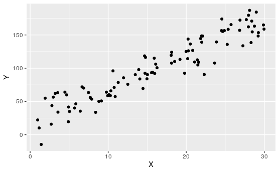
In order for this to be a sensible task to embark on, the underlying variables should actually have a linear relationship, or we should have good reason to think that they have a linear relationship.
It's sensible for the monthly profit of a company (with one product) to coincide with how many units they sold, since there is a fixed price per unit.
It is not sensible for the areas of squares to have a linear relationship with the length of sides, since areas are the squares of sides, which gives a quadratic relationship.
Activity 7.1.2. Which are Linear?
Of course, when we don't yet understand what the relationship between variables are, or we are dealing with new variables, it may not be clear if they have linear relationships. In this case, our best approach is to look at samples, and try to eyeball which have linear, or linear-ish relationships.
(a)
Determine which of the following appear to have linear relationships.
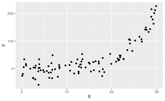
Of course, none of these are perfectly linear. That's usually not the case when dealing with real data.
Definition 7.1.9. Correlation Coefficient.
Given a set of data points \((x_1, y_1), \ldots, (x_n, y_n)\) the correlation coefficient is a statistic \(R, -1\leq R\leq 1\) which measures the strength of the linear relationship between \(x\) and \(y\text{.}\)
\(R=1\) or \(-1\) denotes data that is perfectly aligned with a positive or negative sloping line respectively. The sign of \(R\) gives you the direction of the relationship: positive or negative. The magnitude or distance from 0 determnines the strength of the relationship: weak if close to 0, strong if close to -1 or 1.
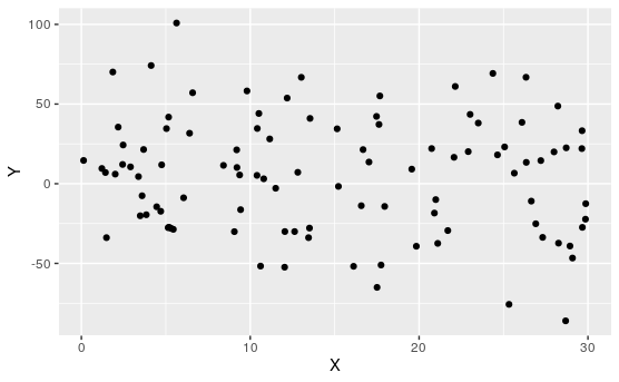
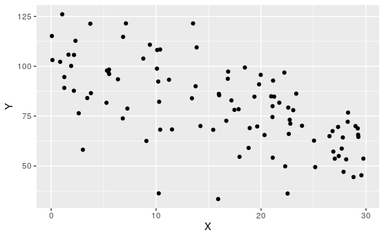
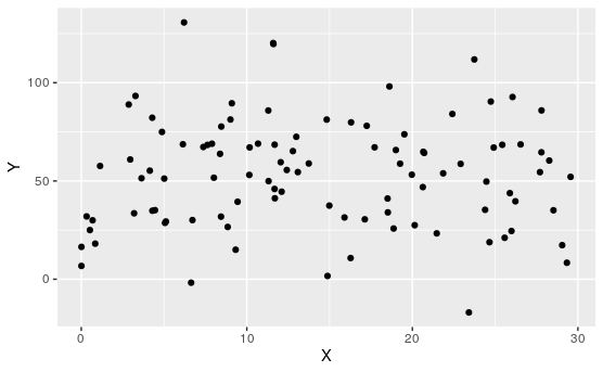
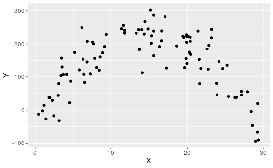
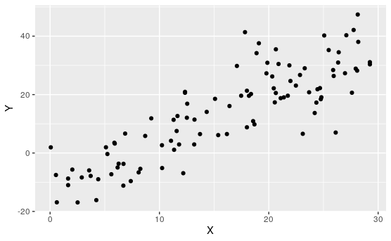
Activity 7.1.3. Match the Plot to \(R\).
For each of the following, match the scatterplot to the correlation coefficient:
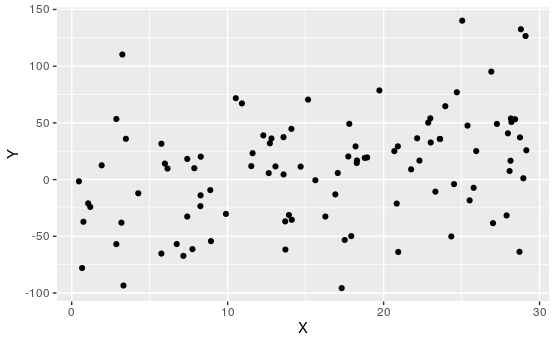
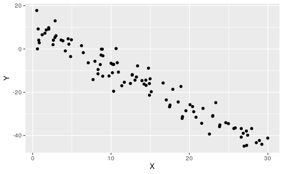
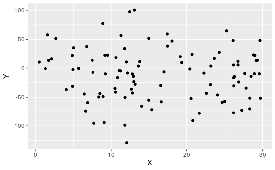
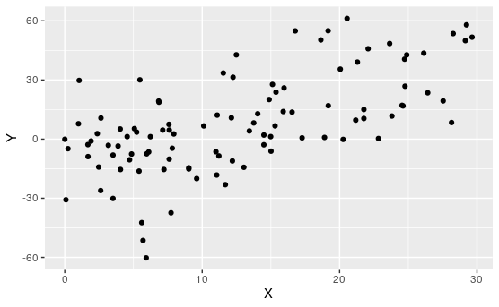
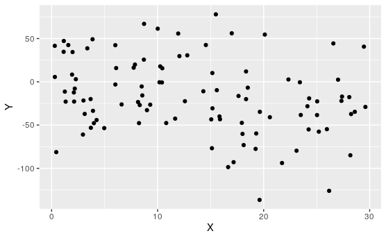
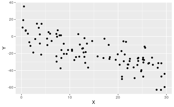
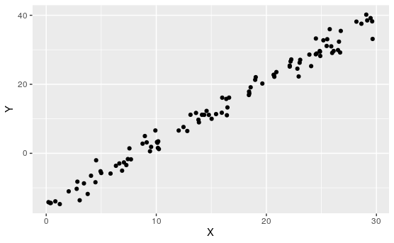
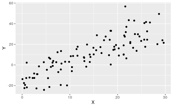
\(\displaystyle R\approx 0.99\)
\(\displaystyle R\approx 0.85\)
\(\displaystyle R\approx 0.65\)
\(\displaystyle R\approx 0.35\)
\(\displaystyle R\approx 0\)
\(\displaystyle R\approx -0.28\)
\(\displaystyle R\approx -0.38\)
\(\displaystyle R\approx -0.75\)
\(\displaystyle R\approx -0.97\)
Remark 7.1.19. Computing the Correlation Coefficient.
\(R\) can be computed
where \(\bar{x}, \bar{y}\) are the mean of the \(x\) and \(y\) variables, and \(s_x, s_y\) are the sample standard deviations.
We won't go through the details of this computation or it's derivation. The main take away is \(\left(\frac{x_i-\bar{x}}{s_x}\right), \left(\frac{y_i-\bar{y}}{s_y}\right)\) measures the distance of the data points from their mean, scaled by the deviation. If \(x_i\) is above (or below)\(\bar{x}\) whenever \(y_i\) is above (or below) \(\bar{y}\text{,}\) then these terms are positive and the sum is large and positive. If one is above whenever the other is below, these terms are negative and the sum is large and negative. If it's a mix, then the positive and negative terms cancel and you are close to 0.
Remark 7.1.20.
We often square \(R\text{:}\) \(R^2\text{,}\) to remove the sign and just to measure the strength of the linear relationship. \(R^2\) explains what proportion of the response variable can be explained by the explanatory variable. This can range from \(R^2=1\) or 100% of the explanatory variable is explained by the response variable, to \(R^2=0\) the explanatory variable has no impact at all on the response variable.
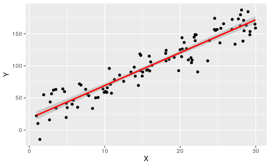
Subsection 7.1.2 Best Fit Lines
Exploration 7.1.4. Best Fit.
For the following scatter plot:
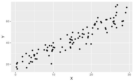
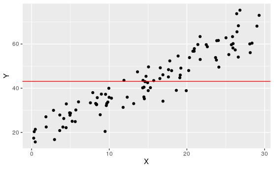
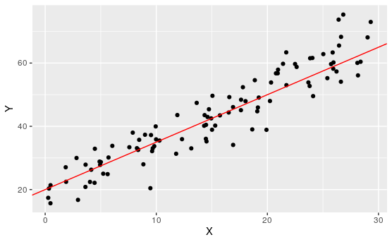
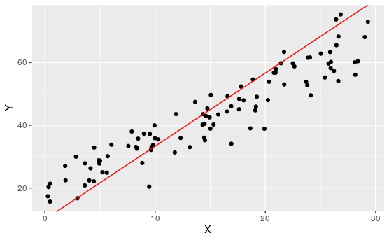
Remark 7.1.24.
Of course, none of these lines perfectly represent all of these points, no line could. There will neccesarily be some overshoot and undershoot. We want to find a line that minimizes this.
Given a point in the scatterplot \((x_i, y_i)\text{,}\) and a line \(y=\beta_1x+\beta_0\text{,}\) let \(\hat{y}_i:=\beta_1x_i+\beta_0\text{.}\) This is the value of \(y\) that the line predicts. Call \(e_i=y_i-\hat{y}_i\) the residual or error of the line. This is the difference between what the model predicts and the actual value.
Our goal is to minimize
the squared some of errors (to remove sign).
Activity 7.1.5. Least Squares Line.
The least squares line is the line which minimizes the sum of squared errors (hence the name).
(a)
Consider the following scatterplot and a proposed regression line. Note that the squared errors are on display, as is S the sum of the squared errors.
Adjust the line to get S as small as possible.
(b)
How well does this line now approximate the scatterplot?
Remark 7.1.25. Finding the regression line.
The parameters for a least square line can be computed as follows:
Recall that the slope of a line is change in \(y\) over change in \(x\text{.}\) How much a variable changes (ignoring direction) can roughly be thought of as it's variation. So we have
\begin{equation*} \beta_1=\frac{s_y}{s_x}R. \end{equation*}The “change” in \(y\) over the “change” in \(x\text{,}\) modified for sign and strength of the relationship.-
While we can't expect every data point to lie on this line, we should expect that “on average” that we can predict \(y\) with \(x\text{.}\) Thus:
\begin{align*} (y-\bar{y})\amp=\beta_1(x-\bar{x})\\ y\amp=\beta_1x-\beta_1\bar{x}+\bar{y}\\ y\amp=\beta_1x+(\bar{y}-\beta_1\bar{x}). \end{align*}Thus:
\begin{equation*} \beta_0=\bar{y}-\beta_1\bar{x}. \end{equation*}
Activity 7.1.6. Linear Regression and Technology.
In practice, we use technology to perform linear regression. Let's recall the data from Activity 7.1.5:
(a)
Enter this data into the columns x_1, y_1:
How do B_1, B_0 compare to the B_1, B_0 from Activity 7.1.5?
(b)
What is the correlation coefficient \(R\)=r? What does this tell us about the relationship between \(y\) and \(x\text{.}\)
(c)
What is \(R^2\text{?}\) What does this tell us about the relationship between \(y\) and \(x\) according to Remark 7.1.20.
(d)
Let's use R to do the same. Run the following code to produce a dataframe dummydata with variables x1 and y1.
(e)
Run the following code to create a linear model for this data, and save it as dummymod.
(f)
Run the following code to show the correlation for this model.
How does this value compare to what you found in (a)?(g)
Run the following code to plot the scatterplot and the least squares line.
Activity 7.1.7. Possum Regression.
We now return to the question from Exploration 7.1.1 and see if we can give a more precise answer.
(a)
Run the following code to create a linear model for head_l, as a function of skull_w and save it as possummod.
(b)
Run the following code to show the correlation for this model.
(c)
What is \(R^2\text{?}\) What proportion of the head length is determined by the skull width. (See Remark 7.1.20.)
(d)
Run the following code to plot the scatterplot and the least squares line.
(e)
Run the following code to show a summary of possummod.
(f)
Run the following code to show a summary of possum.
possum and repeat the above.