Chi-Squared Test and Goodness of Fit (C3)

Section 5.3 Chi-Squared Test and Goodness of Fit (C3)

In previous sections, we discuss the proportion of a categorical variable which takes on a certain value. In this section, we look at the distribution of a sample of a categorical variable across all it's values. In particular, we see if a sample can plausibly come from a given distribution for the variable.

Exploration 5.3.1. Racial Demographics and Jurors.

A small town is 70% White, 15% Black, 10% Hispanic and 5% Asian. In a random sample of 300 jurors from the town, we say that 237 were White, 26 were Black, 24 were Hispanic and 13 were Asian.

(a)

If you randomly selected 300 people from a town that is 70% White, 15% Black, 10% Hispanic and 5% Asian, what are the expected values for the number of White, Black, Hispanic and Asian people to be selected?

(b)

How do these numbers compare to the juror sample?

(c)

Run the following code to simulate selecting 300 random people from the town, and plotting a barchart of the racial demographics.

(d)

Run the following code to summarize the racial demographics of your simulated sample.

How does these values compare to what you found in (a)? To the juror sample?

There is a clear follow-up question to be asked here. “Does the jury pool match the demographics of the town?” Certainly, a random sample of 300 people need not match the expected demographics exactly. But the more it deviates from the town demographics, the less likely we are to be inclined to think that these demographics match.

In the language of Hypothesis Testing, this section is focused on null and alternative hypothesis of the following form: Given a proposed distribution for a categorical variable...

\(H_0\text{:}\)“The sample comes from the proposed distribution.”
\(H_A\text{:}\)“The sample does not come from the proposed distribution.”

Subsection 5.3.1 The chi-square distribution

Remark 5.3.1.

So suppose we did assume the null hypothesis that a sample comes from a certain distribution. We essentially want to develop a measure of how far this sample deviates from the proposed distribution. If it's a little, it's plausible it may come from the null distribution. If it's a significant deviation, we reject the idea that this is the distribution from where the sample comes.

Suppose that we did have a random variable with \(k\) possible outcomes: \(O_1, \ldots O_k\text{,}\) and a sample with \(n_1, n_2, \ldots, n_k\) data points corresponding to each outcome. Note that the total size of the sample is \(n=n_1+\cdots n_k\text{.}\) Let \(E_1, \ldots, E_k\) denote the expected number of outcomes for each value, if a sample of size \(n\) were taken from the proposed distribution.

\begin{equation*} \begin{array}{|r|c|c|c|c|} \hline \text{Outcomes:} \amp O_1 \amp O_2 \amp \cdots \amp O_k \\ \hline \text{Sample Frequency:} \amp n_1 \amp n_2 \amp \cdots \amp n_k \\ \hline \text{Expected Frequency:} \amp E_1 \amp E_2 \amp \cdots \amp E_k \\ \hline \end{array} \end{equation*}

We then compute the test statistic for the \(i\)th value is

\begin{equation*} Z_i=\frac{n_i-E_i}{\sqrt{E_i}}. \end{equation*}

Then we compute

\begin{equation*} \chi^2=Z_1^2+\cdots Z_k^2=\frac{(n_1-E_1)^2}{E_1}+\cdots+\frac{(n_k-E_k)^2}{E_k}. \end{equation*}

This removes the distinction between over and undershooting the expectations, and sums the adjusted error for all the values, which gives a measure for the “total” deviation from the theoritical expectation. (Think Activity 1.5.3, Definition 1.5.1.)

Activity 5.3.2. Racial Demographics and Jurors: \(Z\) and \(\chi^2\) Statistics.

Recall from Exploration 5.3.1 that we have a sample of size \(n=300\) where 237 are White, 26 are Black, 24 are Hispanic and 13 are Asian. We also have a proposed distribution: 70% White, 15% Black, 10% Hispanic and 5% Asian.

(a)

Recall that \(n_1=237\) White jurors in the sample, let \(E_1\) denote the expected number of White jurors found in Exploration 5.3.1 (a). Use Remark 5.3.1 to compute \(Z_1\text{.}\)

(b)

Recall that \(n_2=26\) Black jurors in the sample, let \(E_2\) denote the expected number of Black jurors found in Exploration 5.3.1 (a). Use Remark 5.3.1 to compute \(Z_2\text{.}\)

(c)

Recall that \(n_3=24\) Hispanic jurors in the sample, let \(E_3\) denote the expected number of Hispanic jurors found in Exploration 5.3.1 (a). Use Remark 5.3.1 to compute \(Z_3\text{.}\)

(d)

Recall that \(n_4=13\) Asian jurors in the sample, let \(E_4\) denote the expected number of Asian jurors found in Exploration 5.3.1 (a). Use Remark 5.3.1 to compute \(Z_4\text{.}\)

(e)

Use Remark 5.3.1 to compute \(\chi^2\text{.}\)

Activity 5.3.3. The \(\chi^2\) Distribution.

As in other hypothesis tests, we are concerned with computing a \(p\)-value: a probability we see results as extremal as ours or more if we assume the null. We do this by computing areas under the \(\chi^2\)-distribution. The \(\chi^2\)-distribution has but one parameter: the degrees of freedom.

(a)

Adjust the degrees of freedom d_f from 1 through 20. What do we notice about the distribution of the curve as we make these asdjustments?

(b)

The following graph computes the area of a tail where \(\chi^2=1, d_f=1\text{:}\)

Compute the area of the tail where \(\chi^2=8, d_f=5\) by adjusting C_hisquared and d_f.

(c)

Run the following to compute the area of the tail where \(\chi^2=8, d_f=5\text{.}\)

(d)

Use any method to compute the area of the tail where \(\chi^2=4, d_f=4\)

Subsection 5.3.2 Hypothesis Testing and \(\chi^2\)

Remark 5.3.2. Steps to \(\chi^2\) Hypothesis Testing: Goodness of Fit.

Given the set of hypothesis:

\(H_0\text{:}\)“The sample comes from the proposed distribution.”
\(H_A\text{:}\)“The sample does not come from the proposed distribution.”

We compute the \(p\)-value to be the area of the tail on the \(\chi^2\) distribution corresponding to the \(\chi^2\) value computed via Remark 5.3.1 and with \(k-1\) degrees of freedom (recall that \(k\) is the number of possible values of the categorical variable.)

As in other hypothesis testing scenarios, the \(p\)-value measures the probability that, if we assume the null hypothesis, that we see values as or more extreme than what was observed.

We then reject or accept the null based on the level of significance \(\alpha\) which is as before usually 0.05 or 5%. If the \(p\)-value is less than \(\alpha\text{,}\) we reject the null hypothesis, otherwise we accept it. In this context, accepting the null is to say the sample could plausibly come from the proposed distribution. If we reject that then we say it is implausible that it does.

Activity 5.3.4. Racial Demographics and Jurors.

Recall from Activity 5.3.2 that we have a sample of size \(n=300\) where 237 are White, 26 are Black, 24 are Hispanic and 13 are Asian. We also have a proposed distribution: 70% White, 15% Black, 10% Hispanic and 5% Asian.

We also note that since each juror could be one of 4 races, that \(k=4\text{.}\)

(a)

Compute the number of degrees of freedom.

(b)

Using the \(\chi^2\) value found in Activity 5.3.2 and the degrees of freedom, compute the \(p\)-value.

(c)

State the meaning of the \(p\)-value within the context of this problem in a complete sentence.

(d)

If we had a level of significance \(\alpha=0.05\text{,}\) do we reject the null hypothesis?

(e)

Is it plausible that the juror racial demographics is identical to that of the town?

Activity 5.3.5. \(\chi^2\)-testing with Technology.

Your main task as a statistics practioner is to understand and interpret the results of computation. We prefer to let machines do the actual computations as much as possible. Here we will use technology to simplify the process of computing \(p\)-values.

(a)

In O_bs=[], enter in the observed racial demographics from Exploration 5.3.1: 237, 26, 24, 13. Then in E_xpectedproportions=[], enter in the proposed distribution from Exploration 5.3.1: 0.7, 0.15, 0.1, 0.05.

What is the \(p\)-value? How does it compare to what you found in Activity 5.3.4?

(b)

Run the following code, noting the first vector is the vector of racial demographics, and the second vector is the proposed distribution, to compute a \(p\)-value.

What is the \(p\)-value? How does it compare to what you found in Activity 5.3.4?

Activity 5.3.6. Skittle Color Distributions.

Skittles come in 5 colors. Red, Green, Orange, Purple and Yellow. Are the Skittle colors evenly distributed? One of your friends says yes, another disagrees.

Hint. Desmos

(a)

State a null hypothesis for this \(\chi^2\) test.

(b)

State an alternative hypothesis for this \(\chi^2\) test.

(c)

Suppose that you then buy a bag of Skittles, dump it out and count the contents.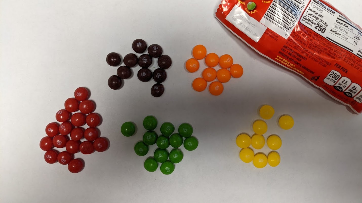

\begin{equation*} \begin{array}{|c|c|c|c|c|c|} \hline \text{Color} \amp \text{Red} \amp \text{Green} \amp \text{Yellow} \amp \text{Purple} \amp \text{Orange}\\ \hline \text{Count} \amp 18 \amp 13 \amp 9 \amp 11 \amp 9\\ \hline \end{array} \end{equation*}

How many Skittles \(n\) are in the bag? How many colors \(k\text{?}\) How many degrees of freedom are there?

(d)

If the null hypothesis were true, what is the expected number of skittles of each color in a sample of size \(n\text{?}\)

(e)

Use any method to compute a \(\chi^2\) statistic.

(f)

Use any method to compute a \(p\)-value.

(g)

State the meaning of the \(p\)-value within the context of this problem in a complete sentence.

(h)

If we had a level of significance \(\alpha=0.05\) do we reject the null hypothesis?

(i)

Is it plausible for Skittle colors to be evenly distributed?

Activity 5.3.7. Male Heights and Normal Distribution.

We examine data from a random selection of adult males to see if their heights are possibly normally distributed.

Run the following code to download the male_heights.csv data set and to display it's variables.

(a)

We begin by examining the heights of adult males in inches. Run the following code to see the sample mean and standard deviation for the heights of adult males in inches, and set them to be m and std respectively.

(b)

IF adult male heights were normally distributed, we would expect it to be approximated by a normal random variable \(X\) with mean \(\mu=m\) and standard deviation \(\sigma=std\text{.}\) Confirm that if we subdivide a normal distribution into intervals of length \(std\text{,}\) we would have:

\begin{align*} P(X\lt m-3std)\amp \approx 0.0014\\ P(m-3std\leq X\lt m-2std)\amp \approx 0.0214\\ P(m-2std\leq X\lt m-std)\amp \approx 0.1359\\ P(m-std\leq X\lt m)\amp \approx 0.3413\\ P(m\leq X\lt m+std)\amp \approx 0.3413\\ P(m+std\leq X\lt m+2std)\amp \approx 0.1359\\ P(m+2std\leq X\lt m+3std)\amp \approx 0.0214\\ P(X\geq m+3std)\amp \approx 0.0014 \end{align*}

Figure 5.3.4. A normal curve segemented into lengths of one standard deviation.

Hint. Desmos

(c)

Run the following code to compute the actual number of adult males were less than \(m-3std\) inches.

(d)

Run the following code to compute the actual number of adult males whose heights were between \(m-3std, m-2std\) inches.

(e)

Edit and run the above code for the remaining intervals, and record the number of adult males within them.

(f)

Edit and run the following code to run the \(\chi^2\) goodness of fit test to see if the number of occurences in each interval corresponds to the theoritical value.

(g)

State a null hypothesis for this \(\chi^2\) test.

(h)

State an alternative hypothesis for this \(\chi^2\) test.

(i)

State the meaning of the \(p\)-value within the context of this problem in a complete sentence.

(j)

If we had a level of significance \(\alpha=0.05\) do we reject the null hypothesis?

(k)

Is it plausible for adult male heights to be normally distributed?

(l)

Run the following code to plot a histogram of the adult male heights in inches and see how well a normal distribution matches this distribution.